7. Description of Sheets

7.1. Main

Set the model path, reload model data to memory, and select active countries for querying

Model Folder path of the MESSAGE model to be connected to the SPLAT interface

Main Region name of the MESSAGE model to be connected to the SPLAT interface

Region Active? list of sub-regions (countries) to be loaded into memory

Scenarios to Load list of currently specified scenarios in the main region, and to specify the scenarios to be loaded into memory

Country Name country codes in the MESSAGE model

Description country names expanded

Power Pool the powerpool a country belongs to

TimeSlices/Load Regions number of time slices modelled per year

# Demands number of demand components

# Technologies number of technologies in country

# Constraints number of constraints in country

Scenarios name of scenarios

Discount Rate discount rate of technologies

Reload Global import model data stored in adb and ldb files into memory, perform various calculations.

Refresh all Sheets refresh data sheets (yellow sheets) for reloaded subregions and scenarios

Save all Scenario Files using SPLAT formatting save all model (adb and ldb) files using excel-SPLAT formatting for selected subregions (use this after making a change with MESSAGE interface) If this button is pressed the MAINa ldb files will also be updated if MAINa is selected, to exclude interconnectors for subregions that are not selected below.

7.2. Input Sheets

This section contains the list of parameters (along with parameter code, their unit and definitions) present in each input sheet in the SPLAT interface.

Note

The parameter values refer to the value of the parameter for the given country for the given scenario for the given year(s).
Time series data can sometimes be inserted for small number of years and SPLAT will interpolate it linearly for missing years.
All costs must be given in common base year (e.g. CMP model adopted 2019 base year.)

7.2.1. Demand

Parameter	Unit	Definition
SentOut Demand	GWh	Demand seen by central generation before entering transmission and distribution grid.

7.2.2. PeakDemand

Parameter	Unit	Definition
SentOut Peak Demand	MW	The aggregate peak demand of the country for the specific year. Sectoral final electricity demand can also be entered.

7.2.3. Transmission and Distribution

The transmission and distribution sheets are used to review or modify transmission and distribution technologies parameters as per the definitions in the TechnologySets sheet (see section below).

Note

If the user wants to model with “sent-out” demand (see demand), transmission efficiency must be set to 100%, and investment costs set to a small value. In the default configuration there is no distribution technology specified for “Sent-out” electricity.
If a user specifies values both in the Constant column, as well as under milestone year columns, only the constant value will be used to update the MESSAGE model and the other values will be ignored.

Parameter	Unit	Definition
Efficiency	%	Efficiency of the transmission or distribution system.
Overnight Cost	$/kW	The cost of a construction project if no interest was incurred during construction, as if the project was completed “overnight”. Values are given in constant prices of base year.
Fixed O&M Cost	$/kW	Annual fixed operating and maintenance cost in prices of base year.

Note

For distribution, values need to be entered for urban, rural, industry and commerce distribution types.

7.2.4. FuelPrices

Parameter	Unit	Definition
Variable Cost	$/GJ	Refers to the price of the given fuel or resource. Variable cost for supply of wind, solar and hydro, and extraction of bagasse are set as zero.

7.2.5. GenericTech and SpecificTech

The GenericTech sheet displays generic technology parameters.

The SpecificTech sheet is used to review and update site specific power generation technology parameters that are constant over time. The SpecificTech sheet has an extra button: Add missing Tech, which allows the user to add new site specific technology to the MESSAGE model that is linked. Currently this action makes the addition by copying the technology parameters of a generic technology of the same technology type as specified by the first 6 characters in the technology name. A new technology will be automatically added to all active scenarios. A MESSAGE technology code is created automatically based on the input and output commodities (as specified by the associated generic technology) and the already existing technologies having the same inputs and outputs. Once a new technology is added, its parameters must be updated using the Update Model Data button.

Parameter	Parameter Code	Unit	Definition
Input/Fuel	Par_minp		The fuel that is consumed by a technology and it’s level in the energy system. e.g., Gas/Primary is the input fuel for gas co-fired technology.
Output	Par_moutp-ef		The output of the given technology. e.g., Electricity/Secondary is the output of gas co-fired technology.
Minimum utilization rate	Par_minutil		Fraction of time in a year the technology must be used/dispatched. The value ranges between 0 and 1, and is 0 for most technologies.
First year	Par_fyear		First year in which the technology can be built in the future.
Life	Par_pll	year	Operational life of the technology.
Efficiency	Par_moutp	%	Output to input ratio of the given technology.
Plant factor	Par_plf		A technology has a profile if one of its inputs/outputs has a profile. If a technology has profile (e.g., hydropower), plant factor is the maximum availability of a technology in each load region. If the technology has no profile, plant factor is the maximum availability of a technology per year. The availability gets scaled by plant factor. Leave equal to 1 or blank to use availability as specified by profile.
Operation time	Par_optm		Fraction of time in a year the technology can be in operation.
Plant Status**	Par_status		Can be existing, committed or candidate depending on the status of the plant.
hist.string**	Par_hisc	year1 MW1 year2 MW2	Year of installation of the technology, and its capacity at the time. If a plant is installed over multiple years in different steps, it can be specified as year1 MW1 and year2 MW2 for unit1 and unit2 respectively.
Total Capacity Upper Limit**	Par_bdi_up		Total capacity upper limit of the technology throughout its lifetime.
Load Curve**			This is not an input parameter, but a flag to indicate whether a load profile (or curve) is associated with this Technology. 1 = yes, 0 = no.

Note

The profiles/load curves are calculated by SPLAT based on the hourly values (8760) present in *.tit file in data folder. They are stored in the adb, ldb and ldr files. The reason for not having them in the spreadsheet is that they vary depending on the load region/timeslice definition (e.g. large model/small model) and are would be very difficult to manage effectively in a spreadsheet.
** Parameters relevant to SpecificTech sheet only.

7.2.6. GenericTechCosts and SpecificTechCosts

These sheets display the cost parameters that are either constant or change over the model horizon.

Parameter	Unit	Definition
Overnight Investment Cost	$/kW	Overnight costs in constant prices of base year.
Fixed O&M Cost	$/kW	Fixed operation and maintenace cost for the given technology.
Variable O&M Cost	$/MWh	Variable operation and maintenance cost for the given technology.

7.2.7. SpecificTechHydroDams

The approach to define hydro dam technologies in SPLAT is given in Hydro Dam section. The parameters used to define them are given below:

Parameter	Parameter Code	Unit	Definition
Description	Par_Descr1		Description of dam hydropower technology. This does not affect any SPLAT functionalities.
Corresponding River Tech	Par_river_tech		Technology code: {CountryCode}RIDM_{ProjectName}}
River Capacity Max Flow	Par_bdi_up_R	MW	This is a total capacity limit for the corresponding river technology to define the river’s max flow in MW derived from max flows in m3/s.
Dam Storage Constraint Long Name	Par_storage_con		Technology code: D_{CountryCode}HYDM_{ProjectName}
Dam Storage Constraint Short Name			Named as D001, D002, and so on based on dam hydropower technologies in the country.
Available dam storage capacity	Par_storage_up	MWyr	Storage volume that can be used by the power plant in energy terms. This value in MWyr is derived from the reservoir size (million m3), the energy per unit volume (MJ/m3) and an assumption around minimum volume for reservoir unless this information is available.
River-storage coefficient	Par_river_coef		This is the coefficient for the storage associated with this power plant. +1 means that Each MWyr (or GJ) that flows out of the River Technology will increment the storage level by 1 MWyr or 1 GJ
Storage-PP coefficient	Par_stor_coef		This is the coefficient for the storage associated with this power plant. -1 means that Each MWyr (or GJ) that flows out of the PP Technology will decrease the storage level by 1 MWyr or 1 GJ

7.2.8. Battery&PumpStorage

The approach to define battery and pump storage technologies in SPLAT excel interface is given in Batteries and Pump Storage section. In the SPLAT MESSAGE modelling framework, the battery storage technologies are modelled as generic technologies, unless there are any existing or committed projects. The pumped hydro storage technologies are modelled as non-generic technologies. The storage capacity in terms of MW is based on the result of the optimization process (the total capacity upper limit can be defined in SpecificTech sheet), while the hours of storage already needs to be defined for each technology.

For each storage technology, there is a corresponding proxy technology created automatically by the MESSAGE modelling framework to write the equations. The parameters used to define them are given below:

Parameter	Parameter Code	Unit	Definition
Description	Par_descr1		Includes technology name (Battery Storage or Pump Storage) and storage hours.
Corresponding Proxy Tech			Technology code: {CountryCode}ELPT{StorageHours} for battery storage and {CountryCode}. ELPTPS for pump storage. The proxy technologies are created automatically by MESSAGE framework to write equations
Hours of storage	Par_hrs	hours	Storage hours offered by the techniology.
Storage efficiency	Par_moutp	%	Ratio of energy output by the system to the energy input to the system.
RelationSSLongName			Technology code: SS_{CountryCode}{StorageTechnologyCode}. Storage technology code is ELPT for battery storage and ELPTPS for pump storage.
RelationSSShortName			Named as SS01, SS02, and so on based on storage technologies available in the country.
Proxy Capacity Constraint Long Name			Technology code: PC_{CountryCode}{StorageTechnologyCode}
Proxy Capacity Constraint Short Name			Named as PC01, PC02, and so on based on storage technologies available in the country.
Rel.SS-Proxy Constraint Long Name			Technology code: PS_{CountryCode}{StorageTechnologyCode}
Rel.SS-Proxy Constraint Short Name			Named as PS01, PS02, and so on based on storage technologies available in the country.
ST_Act.1.-SS Coefficient			Used in balance equation. -1 in Activity 1refers that the technology will take 1 unit of energy from the system.
ST_Act.2.-SS Coefficient			Same as cycle efficiency. Used in balance equation. 0.9 in Activity 2 refers that 0.9 unit of energy from the system will be stored by the technology.
ST_Cap-PC Coefficient			Storage technology contribution to reserve margin.
PT_Cap-PC Coefficient			Default value for proxy technology.
PT_Act.1.-PS Coefficient			Default value for proxy technology.
SS-PS Coefficient			Default value for proxy technology.

7.2.9. Interconnectors

The interconnectors sheet is used to review and update cross-border interconnector parameters. At a minimum the two interconnecting countries (which must be active) must be specified to view the interconnections between them.

Parameter	Parameter Code	Unit	Definition
Desciption	Par_Descr1		List of possible interconnectors between country 1 and country 2 in the model.
First Year	Par_fyear		First year in which the technology can be built in the future.
Efficiency	Par_moutp		Efficiency of transmission. Assumed 95% or above.
Total Capacity Upper Limit	Par_bdi_up		Maximum possible installed transfer capacity of the interconnectors.
hist.string	Par_hisc		Year of installation of the technology, and its capacity at the time.
Overnight Cost	Par_inv	$/kW	Overnight costs in constant prices of base year.

7.2.10. SpecificCapacityLimits and InterconnectorsCapLimits

Parameter	Unit	Definition
New capacity fixed limit	MW	Fixed limit on new capacity addition of the technology. Same as bdc_fx.
New capacity lower limit	MW	Minimum new capacity addition of the technology. Same as bdc_lo.
New capacity upper limit	MW	Maximum new capacity addition of the technology. Same as bdc_up.
Total capacity fixed limit	MW	Fixed limit on total installed capacity of the technology. Same as bdi_fx.
Total capacity lower limit	MW	Minimum total installed capacity of the technology. Same as bdi_lo.
Total Capacity Upper Limit	MW	Maximum total installed capacity of the technology. Same as bdi_up.

7.2.11. PVZones, WindZones, OffshoreWindZones, CSP6hrZones and CSP12hrZones

The approach to define VRE technologies (solar PV, CSP, onshore and offshore wind) is given in Solar PV, CSP, onshore and offshore Wind section. The parameters needed to define VRE zones are stated in the table below:

Parameter	Parameter Code	Unit	Definition
Description	Par_descr1		Name of PV or Wind Zones within the country.
Total Capacity Upper Limit	Par_bdi_up	MW	Maximum possible installed capacity of the VRE technology within the given zone based on MSR work.
Latitude	Par_lat	degree	Latitude of the given VRE zone.
Longitude	Par_long	degree	Longitude of the given VRE zone.
Offset Investment (connection to road+grid) extension	Par_offsetinv	$/kW	Offset investment to account for connection to road and grid extension for the VRE zones. SPLAT will add that value to what ever value is currently stored for investment cost “inv” with that technology.
Multiplier Investment (according to turbine class)	Par_multinv	factor	Factor to scale investment cost for onshore wind technologies.

Note

Latitute and Longitude data can be stored in the adb files together with the rest of the model input data. It is not used by SPLAT or MESSAGE for anything, but it can be used by results viewers for display on maps (e.g. in Tableau).
For offset investment and multiplier investment parameters, one has to remember to use the pull down option “Reset Investment” in cell F6, when generic costs are updated for whatever reason, or before an update was made in raw MSR data, before re-applying the “Offset Investment”.
The multiplier investment (according to turbine class) parameter is in WindZones sheet only. This categorization doesn’t apply to offshore as it is assumed all offshore wind turbines are of the same class.

7.3. Constraint Sheets

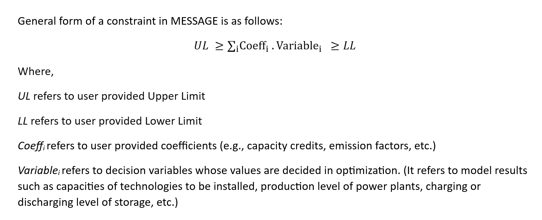
Constraints are linear mathematical equations applicable across several technologies (power plants, storage, transmission, etc. These are user-defined relations to guide a model based on scenario narratives. In MESSAGE, a constraint is defined as a sum-product of a coefficient and variable with user-defined upper or lower limits as shown below:

This section describes the different constraints (including their equations and parameters) present in different Constraint sheets in SPLAT.

7.3.1. ConstraintList

This sheet contains the list of all the constraints in the model which are defined in the following sheets.

7.3.2. PVAnnualBuildLim and WindAnnualBuildLim

These two sheets are used to set annual build limits for solar PV and wind onshore respectively. The equation(s) used in the sheet is as given below:

$\sum\limits_{PV}New\, Capacity\, in\, year\, t_{PV} <= PVBR\, in\, year\, t$

$\sum\limits_{Wind}New\, Capacity\, in\, year\, t_{Wind} <= WindBR\, in\, year\, t$

The equation suggests that the new installed capacity of solar PV or wind for year t should be below the build rates defined in this sheet.

The parameters used in this sheet are as follows:

Parameter	Parameter Code	Unit	Definition
Target (% of peak demand)		% of peak demand	This refers to the country target to meet certain percentage of peak demand by means of given technology. Set as a design decision/suggestion.
Max		MW	Maximum new installed capacity limit for any country in the region. Set as design decision/suggestion.
Min		MW	Minimum new installed capacity limit for any country in the region. Set as design decision/suggestion.
Upper limit	PVBR or WDBR	MW	x = Min value. y = Minimum between Max and VRE capacity target to meet the peak demand. The capacity upper limit is defined as the maximum value between x and y.

Note

The target (% of peak demand), Min and Max values are set as design decision/suggestion. These values could be made larger or smaller. One can also make country specific coefficients by overwriting the formulas for upper limits.

7.3.3. ReserveMarginConstraint

In a power system, generation must always equal consumption. When the balance is disrupted, it can lead to outages and complete black outs. There are many events that might disturb the balance (many of them are stochastic/predictable with probability) such as planned maintenance, unplaneed stops, changes/variations in demand, and changes in supply. Therefore, reserves are needed in the system to make sure that power demand is always met.

Based on the response (reaction time), reserved can be classified as:

Primary reserves: part of operational (running) or fast to activate capacity available to immediately (in seconds) for cover for disturbances.
Secondary reserve: can be operating or cold (not operating) capacity to be activated in minutes (after initial disturbance and activation of primary reserve, secondary reserve is activated, and units are redispatched so to re-activate primary reserve capabilities.)
Tertiary reserve: these are usually back-up units that can be activated in minutes/hours to allow reactivation of secondary reserve capabilities.

In MESSAGE framework, all information about current and future power system is assumed to be known (with 100% certainty), i.e., not stochastic, therefore, production pattern decisions always have to deterministic. When modelling long term development of a power system, an analyst should make sure that the future capacity is sufficient to cover demand during critical periods (usually during peak hours) and to cover other operational needs (e.g., maintenance).

Note

There’s a lot of stochastic behavior in a real system that cannot be captured in the same way within the model.
It is possible to run analysis with various demand and supply availability patterns and model extreme operational conditions.

Reserve margin is the margin of firm capacity that is required above peak demand/load. It ranges usually between 10% to 25% of peak load. For e.g., if a region has 12 GW of firm capacity and 10 GW of peak demand, the reserve margin would be 20%.

Reserve Margin (RM) = (Firm Capacity - Peak Demand) / Peak Demand

The representation of system reserve in MESSAGE modelling framework is as shown below:

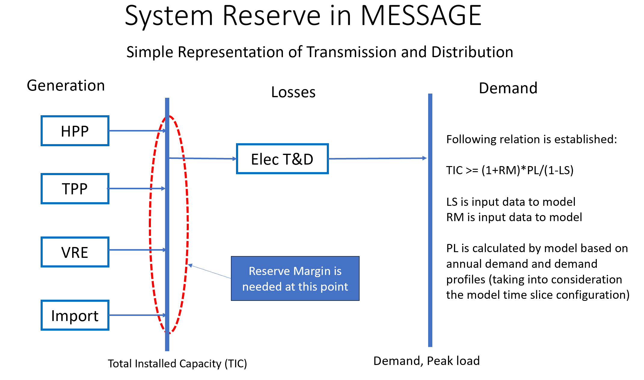
The constraint equation used in the ReserveMarginConstraint sheet is as follows:

$\sum\limits_{PP}(CapacityCredit_{PP} \times Capacity_{PP}) - \dfrac{1+RM}{1-LS} \cdot Capacity_{Ptnd} \geq 0$

where,

PP refers to all applicable power plants.

CapacityCredit_PP and Capacity_PP refer to capacity credit and installed capacity of power plant.

RM = Reserve Margin

Capacity_Pt&d = Size (MW) of transmission and distribution grid used as proxy of peak demand

LS = Transmission Losses

“ConCap_RM” stands for Coefficient applicable on Capacity (MW) and associated to Reserve Margin constraint.

Parameter	Parameter Code	Unit	Definition
RHS Reserve Margin Lower Limit	RM		Set as 0 by default. Minimum RM.
RHS Reserve Margin Upper Limit			Maximum RM. Since the model is solving for least cost, it will not “overbuild” without a good reason for it. We don’t want to disallow overbuild, which setting an upper limit would do. Therefore, it is kept blank.
Reserve Margin		%	Percentage of peak demand. Used to derive capacity credit of transmission.
Tx Losses (for transmission capacity credit)		%	Percentage of transmission losses.
LHS Capacity credit	Concap_RM		Capacity of the technology that is allocted to provide reliable and stable power. It is measured over period of critical conditions, such as peak load.

Note

Unlike build rate constraint, SPLAT requires the user to insert reserve margin constraint as a non time-series constraint i.e., a constant upper or lower limit applied on all years in modelling horizon.

7.3.4. LocalREConstraint

Different countries or regions can have target of achieving certain minimum share RE in the the total power generation by certain year. In the LocalREConstraint sheet, the minimum “target” share of RE (more specifically VRE) technologies in the total power generation is set as a constraint in the model for different years. The equation representing this constraint can be represented as follows:

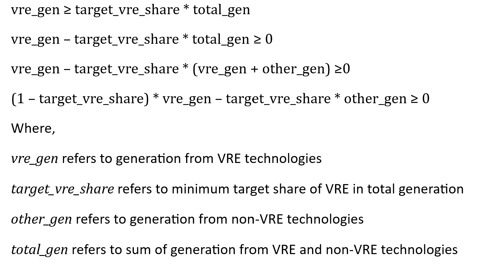
“ConAct_RE” refers to the coefficient of Activity/Generation (GWh) of a power plant technology.

Parameter	Parameter Code	Unit	Definition
RHS RE share lower limit		%	Minimum RE share in electricity supply. Set as 0 by default.
RHS RE Share upper limit		%	Maximum RE share in electricity supply. Left blank by default.
RHS RE target		%	RE target to meet share of electricity demand by given year.
RHS Tx Losses		%	Percentage of transmission losses in given year.
LHS ConAct_RE	ConAct_RE		Set to 1 for RE techs and zero for the others. Backstop is included to avoid infeasibilities in the case where there are not enough technology options to meet the target.
LHS transmission			set to -x for the transmission technology, where x is the RE target share (by energy),

7.3.5. CO2Constraint:

The CO2 emissions constraints are set in more ambitious scenarios. In this sheet, the reduction target for CO2 emissions for different years is set relative to a specific reference scenario. This in turn sets the upper limit on the CO2 emissions from power generation from different technologies. The constraint equation used in the model is as shown below:

$\sum\limits_{PP}CO2_{PP, t} <= MaxCO2_t$

where,

LHS represents the sum of CO2 emissions from power sector in year t.

RHS represents the maximum limit of CO2 emissions from power sector in same year t.

Parameter	Unit	Definition
Reduction target		Target for reducing emissions from power sector relative to reference values (in columns J-N)
RHS Upper Limit	ktCO2	Maximum possible CO2 emissions from the power system.

7.4. ReportGen-Annual

This sheet allows to run the model and get results in annual resolution. The steps are described in Running the model.

7.5. ReportGen-Profiles

This sheet allows to generate Sub-Annual (Profiles) results file. The steps are described in Extracting the results.

7.6. TimeSlices

Displays timeslice definitions (load regions) used in model